Bibliography

1

Johnston L, Atkins MS, Mackiewich B, Anderson M. Segmentation of Multiple-Sclerosis Lesions in Intensity Corrected Multispectral MRI. IEEE Trans Med Ima 1996;15(2):154-69

2

Zijdenbos AP, Dawant BM. Brain Segmentation and White Matter Lesion Detection in MR Images. Critic Rev Biomed Eng 1994;22(5-6):401-65

3

Filippi M, Yousry T, Baratti C, et al. Quantitative assessment of MRI lesion load in multiple sclerosis. A comparison of conventional spin-echo with fast fluid-attenuated inversion recovery. Brain 1996;119(Pt 4):1349-1355

4

Hajnal JV, Oatridge A, Murdoch J, Kasuboski L, Bydder GM, Failure of FLAIR sequences to suppress CSF in the Posterior Fossa: Diagnosis of a Problem and Solution with adiabatic inversion pulses. In Proc. 6th Annual Meeting of the International Society for Magnetic Resonance in Medicine, p. 1350, Sydney, April 18-24, 1998

5

Filippi M, Gawne-Cain ML, Gasterini C, et al. Effect of training and different measurement strategies on the reproducibility of brain MRI lesion load measurements in multiple sclerosis. Neurology 1998;50(1):238-244

6

Mark AS, Atlas SW. Progressive multifocal leukoencephalopathy in patients with AIDS: appearance on MR images. Radiology 1989;173(2):517-520

7

Trotot PM, Vazeux R, Yamashita HK, et al. MRI pattern of progressive multifocal leukoencephalopathy (PML) in AIDS. Pathological correlations. J Neuroradiol 1990;17(4):233-254

8

Bastianello S, Bozzao A, Paolillo A, et al. Fast spin-echo and fast fluid-attenuated inversion-recovery versus conventional spin-echo sequences for MR quantification of multiple sclerosis lesions. Am J Neuroradiol 1997;18(4):699-704

9

Yousry TA, Filippi M, Becker C, Horsfield MA, Voltz R. Comparison of MR pulse sequences in the detection of multiple sclerosis lesions. Am J Neuroradiol 1997;18(5):959-963

10

Gawne-Cain ML, Silver NC, Moseley IF, Miller DH. Fast FLAIR of the brain: the range of appearances in normal subjects and its application to quantification of white-matter disease. Neuroradiology 1997;39(4):243-249

Figure 1: Automated extraction of a medium-sized lesion in two scans acquired consecutively with two head orientations (top: First scan; bottom: Second scan). Crosses on the left indicate several manually-selected seed points, which, given individually as input to the automated algorithm, all yielded the segmented result shown on the right.

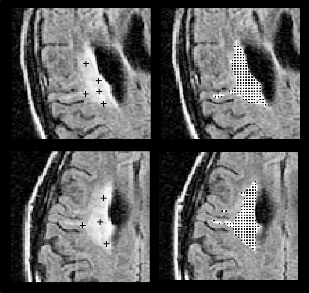Figure 2: (a) Neighborhood used during flooding: the region will grow into volume elements (voxels) with intensities above a threshold $t$ and adjacent to a voxel already known to belong to the lesion (shown in gray), on the same slice as well as on the two adjacent slices. This local flooding is applied recursively until no neighbors above $t$ can be found. (b) The threshold $t$ is adaptively determined for each lesion, by starting from the intensity value at the manually selected seed point, and progressively decreasing the threshold by discrete amounts $a$, until the ratio of flooded lesion volumes obtained for $t$ and $t+a$ becomes greater than a given constant $b$. This typically ocurs as the lesion volume explodes when the threshold becomes sufficiently low as to include voxels in the normal white matter.

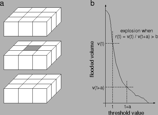Figure 3: Results of the analysis. (a): Lesion volume computed with the automated algorithm correlated well with the volume found with the manual outlining method. (b): However, the difference between manual and automated volumes was often large, particularly for small lesions (for which an error of only a few pixels can be significant). (c)-(e): Experiments with pairs of repositioned scans. Correlation of computed lesion volumes between scans 1 and 2 was excellent for the automated method (c), and also very good for the manual method (d). Volume differences were, however, much lower with the automated method (e; black circles) than with the manual method (e; triangles).

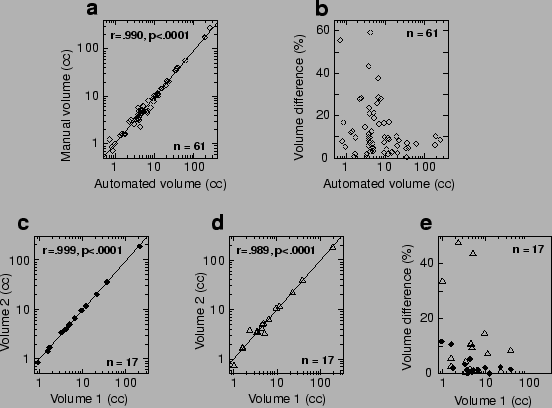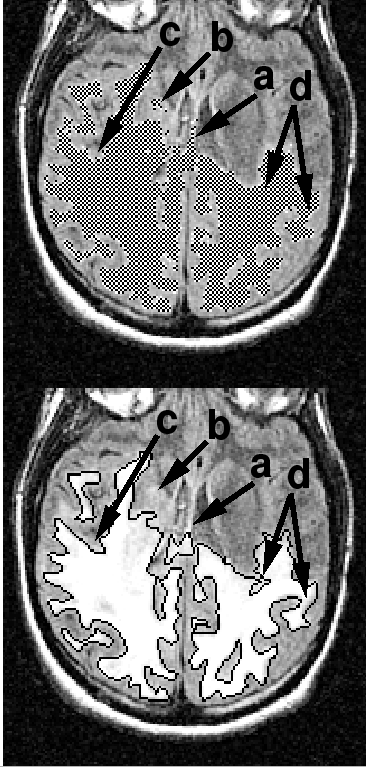
Figure 4: Major sources of discrepancies between the automated (top) and manual (bottom) methods: (a) Imaging artifacts: Hyperintensities at the brain/fluid interface are ambiguous for the automated algorithm; (b) 3D shape coherence: Here the human observer omitted a small island connected to the main body of the lesion in another slice; (c) Small shape irregularities: The manual drawing smoothed out the exact shape of the lesion, which was correctly followed by the automated algorithm; and (d) Inconsistent drawing rules in the manual method, more conservative in some regions (left arrow) than others (right arrow).